
Amael Hinojo,Philippe Christe,Inès Moreno,Robin J. Hofmeister,Gottlieb Dandliker,Fridolin Zimmermann
Journal of Wildlife Management https://wildlife.onlinelibrary.wiley.com/doi/10.1002/jwmg.22307
Abstract
Wildlife conservation and management need accurate methods for population survey and monitoring. Absolute counts of roe deer populations (Capreolus capreolus) are not possible, but the rapid advancement of motion-sensitive camera technologies and new analytical approaches might potentially lead to more precise estimates at lower costs compared to traditional survey methods. We applied spatially explicit photographic capture–recapture models (SCR) in the Lake Geneva basin, Switzerland, from 25 April to 20 September 2018 to estimate roe deer densities in a pilot survey. We investigated the effect of survey duration and camera density on male roe deer density estimates to select the sampling design that produced density estimates with sufficient accuracy and precision at lower costs (i.e., material, fieldwork, data processing, and analyses). Males could be identified based on their antlers, which allowed us to apply SCR to estimate their density. Because females could not be identified individually, we inferred the overall roe deer density (adult and sub-adult roe deer) based on the sex ratio estimated from motion-sensitive camera photos. According to the results of sub-sampling simulations and by taking into account the financial costs associated with fieldwork and analyses, we conclude that 20 motion-sensitive cameras set over 20 nights (i.e., the 20/20 method) is a good compromise to provide reliable estimates of male roe deer density. Furthermore, studies estimating overall roe deer density using SCR and sex ratio estimates should be conducted from mid-August to the end of October just after rutting season and the peak of yearling dispersal, when the movement rates of males and females, and hence their detection probabilities, are similar and when males are still carrying their antlers. This approach was successfully applied in 4 selected study areas with contrasting roe deer management regimes, resulting in overall roe deer density estimates ranging from 3.9 ± 1.3 (SE) deer/km2 forest to 22.5 ± 6.1 deer/km2 forest. Our study provides a valuable and cost-effective approach using photographic SCR methodology and sex ratio information to calculate roe deer density estimates that can be used in management measures such as defining hunting quotas.
Reliable data on population size, density, and structure are cornerstones of effective management and conservation of wildlife populations (Noon et al. 2012, Caravaggi et al. 2016, Pfeffer et al. 2017). Ungulates can be secretive and difficult to observe, particularly in forested areas. Therefore, they are extraordinarily difficult to survey and almost invariably their density is underestimated (Andersen 1953, Pielowski 1984, Ratcliffe 1987). Different methods have been used in ungulate surveys including capture-mark-recapture, transect methods (i.e., kilometer index, spotlight road counts, line transects), pellet-group counts, and index methods such as indicators of ecological changes (i.e., body mass, fecundity, fawn production, measures of skeletal size, browsing index; Morellet et al. 2011, Marcon et al. 2019, ENETWILD consortium et al. 2020). These traditional survey methods are often costly and time consuming and no consensus has been reached on a universal approach for surveys of forest ungulate populations that fulfills the criteria of being easy to apply and cost-effective, and providing reliable estimates (Chećko 2011).
The rapid advance of motion-sensitive camera technologies and new analytical approaches might potentially lead to more precise estimates at lower costs (Bessone et al. 2020, Taylor et al. 2020). If individuals are recognizable, density can be estimated using spatially explicit capture–recapture (SCR) models (Efford 2004; Borchers and Efford 2008; Royle and Young 2008; Royle et al. 2009a, b). Spatially explicit capture–recapture models have already been applied to assess densities of male ungulates including white-tailed deer (Odocoileus virginianus; Beaver et al. 2016, Parsons et al. 2017) and roe deer (Capreolus capreolus; Jiménez et al. 2013) based on their antlers. When some tagged or otherwise marked individuals are available for sampling, both non-spatial (White 1996; McClintock et al. 2006, 2009; McClintock and White 2009) and spatial (Chandler and Royle 2013, Macaulay et al. 2020) mark–resight models can be used. Methods for estimating density from camera data in the absence of individual identification are available but are still in development (Sollmann et al. 2013, Burton et al. 2015, Zimmermann and Foresti 2016). These include calibrated (absolute) abundance indices (e.g., relative abundance index [RAI]; Carbone et al. 2001, O’Brien et al. 2003), the random encounter model (REM; Rowcliffe et al. 2008, 2011, 2016), SCR without individual identities (Chandler and Royle 2013), and a relatively new approach based on distance sampling (Howe et al. 2017, Bessone et al. 2020).
The roe deer is a widespread and common species in Europe. It is a species of interest for its ecological importance (Andersen et al. 1998, Burbaite and Csányi 2009, Martin et al. 2018, Mahmoodi et al. 2020) and its economic value as a hunted species in most European regions (Burbaite and Csányi 2009, Evcin et al. 2019, Spitzer et al. 2021). From the beginning of the twentieth century, European roe deer populations have increased (Andersen et al. 1998) and their distribution range is expanding, notably by colonization of agricultural landscapes (Kaluzinski 1982). The negative effects of high-density roe deer populations are documented including browsing impact on forest regeneration, damages to crops and vineyards, and increased number of traffic accidents (Kjøstvedt et al. 1998, Morellet et al. 2011, Putman et al. 2011, Rodríguez-Morales et al. 2013, Bobrowski et al. 2020). High densities of roe deer have become a controversial topic generating conflicts of interest. Hunters and the general public want higher densities and farmers, winemakers, and foresters aim for lower densities (Meriggi et al. 2008). Consequently, there is an important need for accurate methodologies to survey roe deer, to take adequate management measures (e.g., hunting quotas), and to keep damages, browsing, and vehicle collisions within acceptable limits. Moreover, roe deer is an important prey base for Eurasian lynx (Lynx lynx; Molinari-Jobin et al. 2007) and according to the Swiss Lynx Concept implemented by the Federal Office of the Environment, information on the changes in the number of its main prey species (i.e., roe deer and chamois [Rupicapra rupicapra]) figures among the management criteria to decide whether lynx can be regulated in a given management compartment.
We conducted a pilot survey to investigate the effect of survey duration and camera density on male density estimates in SCR models to select the least costly sampling design that produces density estimates with sufficient accuracy and precision. Subsequently, we applied this design in selected study areas with contrasting roe deer management regimes to estimate overall roe deer densities based on SCR and sex ratio information resulting from camera photos.
STUDY AREA
We conducted this study in 5 different forested areas of the Lake Geneva basin, of which 4 were located in the canton of Geneva and 1 in the canton of Vaud, Switzerland. The Lake Geneva basin is bordered by the Jura Mountains to the northwest, the Swiss Plateau to the north, and the Pre-Alps to the south and to the east. The Lake Geneva basin elevation ranges from 372 m (Lake of Geneva) to 1,080 m (Mont Pèlerin). The region is characterized by moderately continental climate with 4 distinct seasons: spring (Mar–Jun), summer (Jun–Sep), autumn (Sep–Dec), and winter (Dec–Mar). The yearly average temperature was 10.2°C with average temperatures of 2.3°C during winter and 18.2°C during summer. The average annual precipitation was 1,005 mm/year (Federal Office of Meteorology and Climatology 2022). In addition to roe deer, other ungulate species in the area included the red deer (Cervus elaphus) and the wild boar (Sus scrofa). The other dominant mammalian species were the hare (Lepus europaeus), the red fox (Vulpes vulpes), and the badger (Meles meles). Large carnivores such as the Eurasian lynx and the gray wolf (Canis lupus) were present only sporadically.
We conducted all surveys between summer and autumn except the pilot survey, which we conducted from winter to autumn. The pilot survey took place in Satigny in the canton of Geneva (Figure 1; 46.22108N, 6.00667E, ~1 km2). We subsequently applied the method in 4 distinct study areas: Versoix (46.299713N, 6.128610E, ~1 km2), Jussy (46.247162N, 6.295851E, ~1 km2), and Chancy (46.136111N, 5.973503E, ~1 km2) located in the canton of Geneva, and Jorat (46.584676 N, 6.658175E, ~1 km2) located in the canton of Vaud. All study areas in the canton of Geneva were bounded by agricultural land, whereas the Jorat study area was surrounded more by forest than agricultural land. While the forests of the study areas in the canton of Geneva were characterized by a mixed forest of downy oak (Quercus pubescens) and European hornbeam (Carpinus betulus), with some patches of pine (Pinus spp.), silver fir (Abies alba), and European spruce (Picea abies), in the study area of the canton of Vaud, the forest was mainly composed of European beech (Fagus sylvatica) with some patches of European ash (Fraxinus excelsior), silver fir, and European spruce. Since 1976 hunting has been prohibited in the canton of Geneva. Only a few control shootings have occurred since 2017, in the surrounding area of Satigny, where roe deer were harvested at a density of approximately 3 deer/km2 forest/year to reduce damage to vineyards. Hunting is permitted in the canton of Vaud. In the surrounding area of Jorat, harvest was approximately 2 deer/km2 forest/year.
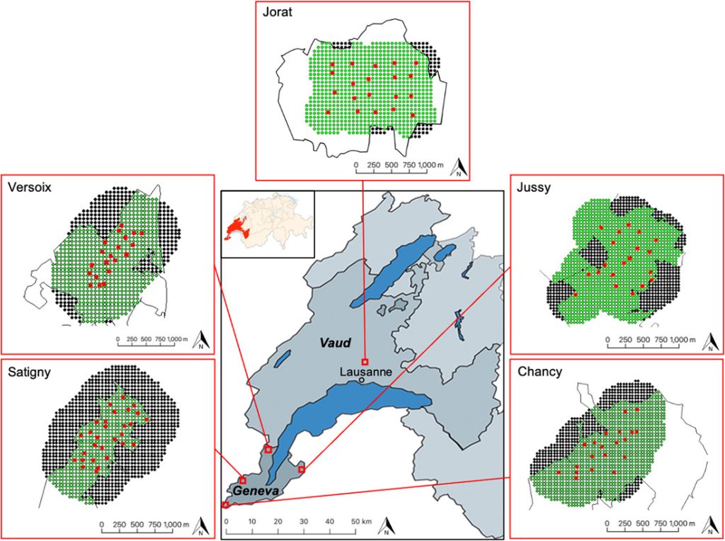
Location of the 5 study areas for estimating roe deer density by motion-sensitive cameras based on spatially explicit capture-recapture models and sex ratio estimates in the canton of Geneva (GE) and Vaud (VD), Switzerland, 2018–2020. We conducted the pilot survey in Satigny (GE) and the 20/20 method in Versoix, Jussy, Chancy (GE), and Jorat (VD). The detailed maps show the state-space of each of the 5 areas surveyed. The red squares show the camera sites, the thin black lines the forest. Dots represent the mask using the trapbuffer method and show the 50-m spaced potential activity centers falling within (green dots) and outside (black dots) the forest. In each study area, the habitat mask corresponds to the area delimited by the green dots.
METHODS
Sampling design
We conducted the camera pilot survey from February to September 2018. Males did not carry fully developed antlers (i.e., annual growing completed and already shed velvets) before the end of April; therefore, we used data collected from 1 May to 20 September to estimate sex ratio based on the information provided by the camera photos and from 25 April to 9 July 2018 (75 nights) to perform SCR analyses.
The size of the study area and camera density was based on other roe deer camera studies (Jiménez et al. 2013) and published home range sizes. Male home ranges can vary seasonally and between populations (Mysterud 1999, Kjellander et al. 2004); the smallest home ranges recorded are about 10 ha (Fruziński et al. 1983, Maublanc et al. 2012). An important requirement of SCR models is the use of spatial recaptures, which would require at least some individuals having access to >1 sampling site within their home ranges. We overlaid a 200 × 200-m (4 ha) grid on the camera study area of 1 km2. We discarded 2 grid cells with ≤50% forest cover and chose an optimal camera site (i.e., principally based on presence signs of roe deer like tracks, beds or browsing damages) in the remaining 23 grid cells. To investigate the effect of camera density, we placed 1 additional site in 6 grid cells among those with the greatest forest cover, resulting in 29 camera sites (Figure 1), which corresponds to 2.9 sampling sites per the smallest male home range.
We attached unbaited cameras to trees at a height of 0.7 m above ground, facing roe deer trails, beds, or damaged vegetation. We used UltraFire™ XR6 cameras (Reconyx®, Holmen, WI, USA) with a passive infrared motion detector, a no-glow infrared flash, and a trigger speed of <1 second. We set cameras to take 3 consecutive photos (image resolution 8MP) followed by a 30-second video (1080P-30 frames/second) at each trigger with no trigger delay between successive triggers (i.e., cameras continue to capture bursts of photos and video as long as movement is detected). We checked cameras monthly to replace secure digital (SD) cards and change batteries when necessary.
Sex ratio estimation and individual identification
We grouped roe deer photos and videos taken during 1 trigger event (i.e., sequence of 3 photos followed by 1 video) into encounters. We only considered the videos when the photos did not allow identification of age, sex, or individual. Roe deer fawns were visually distinct from adults and sub-adults during the study period and were still following their mother. Sub-adults could not be distinguished from adults based on the photos; hence, the abundance estimates refer to adults and sub-adults. We classified each roe deer photographed into 1 of 4 categories based on morphological characteristics (presence of antlers or hair-covered penis sheath) and body proportions: adult and sub-adult males, adult and sub-adult females, fawns (individuals <1 yr old), and roe deer photos of too poor quality to allow identification of sex and age. We considered consecutive photos of roe deer as independent encounters when there was an interval of ≥10 minutes between them except in the following 2 cases: consecutive photos of 1 male followed by another one, and 1 roe deer followed by an individual of the opposite sex or different age category (fawn vs. adult and sub-adult roe deer), in which the 2 encounters were considered as independent even if they were taken <10 minutes apart. With groups of ≥2 roe deer, we estimated the group size including the number of adult males, adult females, and fawns based on the photos that resulted from a trigger and possible subsequent triggers without delay. We assigned the group size to each independent encounter of individual roe deer that belonged to the same group. We did not use fawns in the subsequent analyses because of their low detection rate. When possible, we identified females based on natural marks resulting from the annual molt in spring, which are not uniform over the body. We identified males of each encounter based on their antlers (shape, number of points, length, curvature, and top, back, and brow points morphology) and other natural markings (e.g., forehead color in daylight photos; Figure 2). At least 2 independent observers proceeded with the individual identification to ensure objectivity and to check and resolve identification errors (Choo et al. 2020). To facilitate the identification process, we named all identified males according to some specific physical characteristics (e.g., 6 symmetric, bifurcated, small 4 and right long; Figure 2), and classified all their photos by site. When the identification was uncertain, we recorded the reason (blurriness, distance of the individuals to the camera, head covered by the vegetation). We considered only encounters of adult male roe deer that could be unequivocally identified by all observers in the SCR analyses.
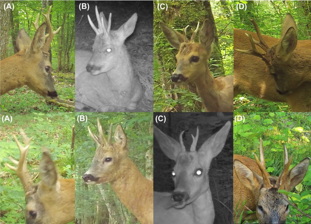
Examples of 4 different male roe deer identified visually from photographs collected during the motion-sensitive camera pilot survey in Satigny, canton of Geneva, Switzerland, 2018. We identified males based on distinctive antler morphology: number or points, length, shape, curvature, and bifurcation height. We named males according to their antler morphology; we named the males in the figure A) 6 symmetric, B) bifurcated, C) small 4, and D) right long.
For each independent encounter, we recorded the following information: site, date, time, category (adult male, adult female, or fawn), group size (number of individuals), name of the male if identifiable, and reason if the individual was not identifiable (e.g., head covered by vegetation, blurriness). We established the sex ratio as the number of independent encounters of males divided by the number of independent encounters of females and males. To show the change in sex ratio estimates in the pilot survey, we divided the study period into 7 periods of 20 nights each and estimated the sex ratio for each period. In view of the definition of the sex ratio used in the present study, its precision can be assessed using parametric bootstrap by drawing 1 million realizations of the number of males from a binomial distribution of the corresponding sex ratio. We defined the RAI as the number of independent encounters of adult and sub-adult roe deer per 100 realized camera nights. For each independent male encounter, we reported site number, date, time, and the identity of the male.
Data analysis
We analyzed data using SCR with a half normal detection function using likelihood inference. Spatially explicit capture–recapture is a set of methods for modeling animal capture–recapture data collected with an array of detectors (Efford 2020), in our case cameras. Animal density is directly estimated using information on capture histories in combination with spatial locations of captures (Efford 2020). The advantage of SCR is that there is no need to define the sampling area, in contrast to the non-spatial methods (Efford and Fewster 2013). We used the secr package (Efford 2020) in R (R Core Team 2019) and the input data of individual male roe deer encounters (i.e., site number, date, time of the encounter, male individual identification), the location of the camera sites, and camera deployment details including dates when cameras were active. We defined a sampling occasion as a time frame of 24 hours starting at noon, which results in 75 sampling occasions for the duration considered in the pilot survey. We used a count detector, which is more likely to be affected by temporal autocorrelation between consecutive encounters of the same individual at the same site than a proximity detector. In our case as defined above, we grouped consecutive photos of the same individual at the same site taken <10 minutes apart into 1 independent encounter.
The last object that needs to be created for secr analysis is the mask to be applied to the array of the camera sites. To compute the mask, we used the trapbuffer method and set the spacing between potential activity centers to 50 m. The mask has to be large enough so that no individual outside of the state-space has any probability of being photo-captured on the array (Royle et al. 2009a, b). A buffer width that is too narrow is likely to produce inflated density estimates; therefore, it is important to determine the buffer width beyond which the density estimates start to stabilize. To determine if the chosen buffer width was large enough (whereon density estimates stabilize), we calculated the SCR densities for 17 different buffer widths ranging from 50–850 m with increments of 50 m based on a null model considering the dates when cameras were active. To get roe deer density estimates per square kilometer of forest, we eliminated all potential activity centers falling in non-forested areas.
We tested different models assuming constant values of animal density (D) and testing different predefined models on the baseline encounter probability (g0) while keeping the movement parameter (σ) constant (Zimmermann and Foresti 2016). We tested the following predefined models that differed by encounter probability: M0 (null), Mt (time factor), MT (time trend), Mb (learned response), Mbk (site-specific learned response), MBk (site-specific transient response), and MK (site transient response; Efford 2020). By assuming a bivariate normal model for detection, the estimated σ can be converted into a 95% home range radius (Repucci et al. 2011).
We generated the full dataset used in the density estimates in the pilot survey from an intensive sampling scheme. To explore how reduced sampling scheme would influence density estimates, bias, precision, number of male individuals, and number of spatial recaptures (i.e., detection of unique individuals at multiple locations in space; Efford and Boulanger 2019), we performed data sub-sampling. To do this, we subsampled camera sites to create scenarios considering 10, 15, 20, 25, and 29 cameras. We also subsampled the sampling occasions by randomly selecting 10, 15, 20, 25, 30, 40, 50, 60, and 70 occasions (nights) within the sampling period of 75 occasions. We considered all possible combinations of number of cameras and occasions, resulting in 45 scenarios, and replicated each 100 times. We then ran each of these subsets of data in the secr package. We used relative standard error (RSE) as a metric for precision. For bias we used relative bias, which is (true—estimate)/true, wherein we considered the density estimate resulting from the full dataset (most intensive sampling scheme [i.e., 29 cameras and 75 sampling occasions]) as the true estimate for the empirical dataset and the level of density defined in the model as the estimate for simulated data following Kristensen and Kovach (2018). In evaluating empirical subsampling for making sampling design recommendations, we set specific targets: 100% model convergence, RSE <25%, and relative bias <12.5%.
For each of the favorable outcomes, we estimated the associated costs in terms of material (cameras = $638 [USD] per unit, locks = $32 per unit, SD cards = $30 per unit, batteries = $34 for 1 camera), fieldwork including mileage costs, data processing, and analyses to determine which of them was the most optimal in terms of costs (Table 1). From a fieldwork point of view, we counted 1 additional field day after 30 days of sampling to change the batteries and SD cards of the cameras and to remove fast-growing vegetation in front of them. For mileage costs we have considered an average of 40 km/field day with a defrayal of $0.95/km. We have considered a salary of $638/day for a technician and $425/day for an assistant according to Swiss rates. A technician conducted all fieldwork and statistical analyses, while a technician and an assistant completed data processing and identification of male roe deer equally.Table 1. Combination of motion-sensitive camera numbers and occasions reaching the fixed targets for male roe deer density estimates using spatially explicit capture-recapture (SCR) models (i.e., 100% model convergence, relative standard error <25%, and relative bias <12.5%) with associated costs including material, mileage, and salary for fieldwork, data processing, and analysis. We collected data during the pilot survey in Satigny, canton of Geneva, Switzerland, 2018.
| Number of cameras | Number of occasions | Sampling effort (nights) | Number of days to set the cameras | Number of days to check the cameras | Number of days to remove cameras from the field | Number of days to process the data | Number of days for male identification | Number of days for SCR analysis | Costs of material (USD) | Costs of mileage (USD) | Salary (USD) | Total costs (USD) |
|---|---|---|---|---|---|---|---|---|---|---|---|---|
| 15 | 40 | 600 | 1 | 1 | 1 | 5.5 | 4 | 1 | $11,970 | $114 | $7,601 | $19,685 |
| 20 | 20 | 400 | 1 | 1 | 3 | 2 | 1 | $14,680 | $76 | $4,572 | $19,328 | |
| 25 | 15 | 375 | 1.5 | 1 | 3 | 2 | 1 | $18,350 | $95 | $4,891 | $23,336 | |
| 29 | 15 | 435 | 2 | 1 | 3.5 | 2.5 | 1 | $21,286 | $114 | $5,741 | $27,141 |
Roe deer density estimates with the 20/20 method
Based on the result of the pilot survey, we concluded that placing 20 cameras for 20 nights in 1 km2 (1 camera/5 ha; i.e., the 20/20 method) was a good compromise to get robust male density estimates. We subsequently sampled 4 selected study areas in different forest massifs with this method: Versoix (25 Jul–14 Aug 2019), Jussy (16 Aug–5 Sep 2019), Chancy (13 Sep–3 Oct 2019), and Jorat (11 Sep–1 Oct 2020). In each of the 4 study areas, we used a regular grid comprising 20 cells of 5 ha each and set 1 camera in each grid cell (Figure 1). In the Jorat study area, we used the camera model Reconyx HC600 Hyperfire, while in the 3 other study areas we used the Reconyx XR6 Ultrafire model. In the Jorat study area, cameras took 5 consecutive photos during a trigger event, while cameras in the other study areas took 3 consecutive photos followed by a video. Based on the experience of the pilot survey, females were not individually identified in the 20/20 method because their natural markings did not provide enough information to identify them univocally. To obtain an estimate for the overall roe deer density in each of the 4 selected study areas, we divided the estimated male density resulting from the SCR analysis by the estimate of the sex ratio in the corresponding study area (i.e., the number of independent encounters of males divided by the number of independent encounters of females and males). In large samples, the sampling distribution of the maximum likelihood estimates of the male density tends towards a normal distribution, with mean equal to maximum likelihood estimation (MLE) and standard deviation equal to the standard error. To get an assessment of the precision of the overall density estimate, we used a parametric bootstrap. We drew 1 random number from the male density ($\bar{x}$ = MLE [density], SD = SE [density]) for each draw from the sampling distribution of the corresponding sex ratio estimate. We then combined the 2 values to obtain 1 draw from the sampling distribution of the overall density. We repeated this procedure 1 million times to get an estimate of the precision of the overall roe deer density in each of the 4 study areas. For all the remaining methodological and analytical steps, we used the same approach as described for the pilot survey.
We conducted all SCR analyses with the R package secr (version 4.3.1) in R (version 4.1.0) and performed sub-sampling using the subset function without replacement (R Core Team 2019, Efford 2020). We created habitat masks with the packages rgdal (Bivand et al. 2019) and prettymapr (Dunnington 2017). We used R packages sp (Pebesma and Bivand 2005), lattice (Sarkar 2008), survival (Therneau 2022), Formula (Zeileis and Croissant 2010), Hmisc (Harrell 2022), plotrix (Lemon 2006), and ggplot2 (Wickham 2016) to produce graphs.
RESULTS
Pilot survey observations
During the pilot survey in Satigny, we recorded 1,239 independent encounters of roe deer during 2,175 of the 2,175 (75 nights × 29 cameras) camera nights (100%) available. A low percentage of these independent encounters (6.9%) comprised roe deer photos of too poor quality to allow the identification of sex and age. These comprised blurred photos (3.1%), individuals too distant from the camera (1.9%), or individuals with the head covered with vegetation (1.9%). Among the independent encounters where age and sex could be identified univocally, most consisted of single adult and sub-adult males (58.8%) and single adult and sub-adult females (24.2%). We observed groups of adult and sub-adult roe deer, which did not exceed 2 individuals in this study, in 3.3% of the independent encounters. The remaining 6.8% corresponds to independent encounters containing a fawn, a group of fawns, a female with a fawn, or a female with 2 fawns. The resulting RAI was 51 roe deer independent encounters/100 realized camera nights. Sex ratio estimates were skewed towards males from 1 May until the beginning of August (∼0.7; Figure 3). In contrast, from 11 August to 20 September the sex ratio estimate was around 0.5 (Figure 3).
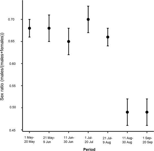
Change in sex ratio estimates calculated as the number of independent encounters of male roe deer divided by the number of independent encounters of male plus female roe deer for every 20-night period of sampling. We assessed the precision (SE) of the sex ratio with parametric bootstrap. We collected data using motion-sensitive cameras during the pilot survey in Satigny, canton of Geneva, Switzerland, 2018.
Pilot survey SCR
We identified 22 male individuals in the pilot survey in Satigny. Individual identification of males was possible in 83.3% of all independent encounters of males. Considering the encounters in which males could be identified at the individual level, most male identifications (92.5%) could be achieved by using only the photos. Nevertheless, we had to rely on the video to identify the individuals in 7.5% of the male encounters. In contrast only 14% of the independent encounters of females could be identified at the individual level, corresponding to 6 females. Consequently, it was not possible to conduct density estimation with SCR for females.
The number of identified males (n = 22; Figure 4) stabilized 43 nights after the beginning of the survey, while the cumulative number of independent encounters increased almost linearly (Figure 4). Twenty out of 22 individuals were already encountered on the nineteenth sampling occasion.
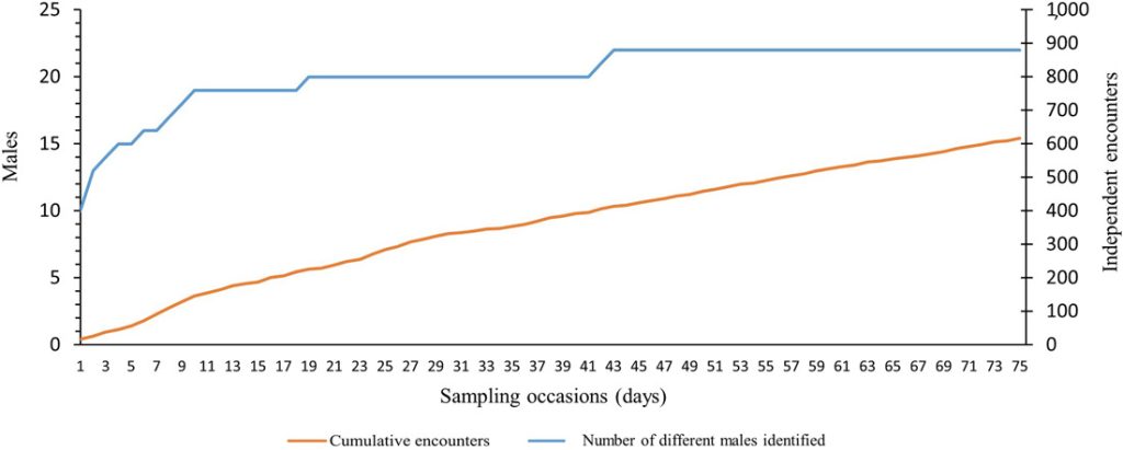
Cumulative number of independent encounters of male roe deer (orange line) and different males identified (blue line) with increasing number of sampling occasions (nights). We collected data using motion-sensitive cameras during the pilot survey in Satigny, canton of Geneva, Switzerland, 2018.
A simple plot of density estimates based on a series of null models integrating the sampling effort showed that SCR density estimates decreased rapidly with increasing buffer width and stabilized when the buffer width was 500 m (Figure A1); hence, we retained this width in the subsequent analysis. Model selection revealed substantial evidence for the site-specific learned response model (Mbk). This model incorporates a site-sensitive change of behavior for individuals after first detection, which implies that if an individual is captured in a specific camera, the probability of a subsequent encounter is decreased (β coefficient = −1.6) and the individual becomes trap shy only for that particular camera. The estimated density from this model amounted to 20.6 ± 4.3 (SE) males/km2 forest, with baseline encounter probability g0 equal to 1.6 ± 0.2. The movement parameter σ of males was 245.1 ± 13.8 m, translating into a 95% home range radius of 599.9 m and a home range size of 113 ha.
Sub-sampling and associated financial costs
The reduction of the sampling effort by sub-sampling the number of cameras and number of nights of sampling reduced the number of males identified, but the decrease was not linear (Figure 5A). The number of males identified varied between 10 ± 2.5 and 22 ± 0 (Figure 5A). The number of spatial recaptures increased with sampling effort (Figure 5B), but the increase was not linear. In general precision increased (RSE decreased) and relative bias (divergence from the estimate with the full dataset) decreased with increasing sampling intensity. When we analyzed the data using smaller subsets, models always converged, except for the 10 cameras and 10 occasions combination, where the convergence was 99%. We achieved RSE < 25% and relative bias < 12.5% with 15 cameras and a minimum 40 occasions (resulting in 600 camera nights in terms of sampling effort), 20 cameras and a minimum of 20 occasions (400 camera nights), and 25 and 29 cameras with a minimum of 15 occasions (375 and 435 camera nights, respectively) in either case (Figure 5C, D). Density estimates increased with increasing number of cameras and number of occasions and stabilized at higher sampling intensity. The number of recaptures increased with sampling effort, but the increase was not linear (Figure B1).
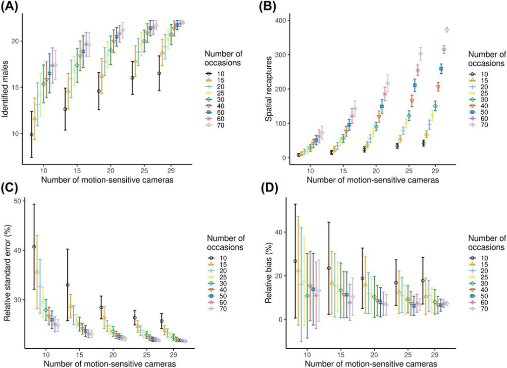
Variation of several statistics (±SD) with increasing sampling effort (from 10 cameras and 10 occasions to 29 cameras and 70 occasions) for male roe deer density estimates using spatially explicit capture-recapture (SCR) models. Models always converged, except for the 10 cameras and 10 occasions combination, where the convergence was 99%. A) The number of identified male roe deer, B) spatial recaptures, C) relative standard errors (RSE), and D) relative bias. Relative bias here measures the divergence in the subsampled estimate from that obtained from the full data set. Frames A and B are a description of raw data, while C and D are parameters estimated using SCR. We collected data using motion-sensitive cameras during the pilot survey in Satigny, canton of Geneva, Switzerland, 2018.
On the basis of the number of days needed to carry out the surveys from the installation of the equipment in the field to the analysis, the scenario that required the fewest working days was the one with 20 cameras and a minimum of 20 occasions, with 8 working days. It was followed closely by the scenario with 25 cameras and a minimum of 15 occasions, with 8.5 working days; the scenarios with 29 cameras and a minimum of 15 occasions required 10 days and the scenario with 15 cameras and a minimum of 40 occasions, required 13.5 working days (Table 1). When looking at the costs (including material, mileage, fieldwork, data processing, and analysis costs calculated according to Swiss rates; Table 1), the least expensive scenario was still the one with 20 cameras and a minimum of 20 occasions amounting $19,328 per survey. It was followed closely by the scenario with 15 cameras and a minimum of 40 occasions, which required $19,685. Next came the scenario with 25 cameras and a minimum of 15 occasions, which required $23,336. Finally, far behind was the scenario with 29 cameras and a minimum of 15 occasions, which required $27,141.
Roe deer density estimates with the 20/20 method
Because of the theft of a camera and some battery failures, the available camera nights of 400 (i.e., 20 sites by 20 nights) were slightly reduced to 397, 387, and 380 realized camera nights, in Jorat, Jussy, and Versoix, respectively (Table 2).Table 2. Summary of the surveys conducted with the 20/20 method to estimate roe deer density using motion-sensitive cameras based on spatially explicit capture-recapture models (SCR) and sex ratio estimates in Versoix, Chancy, and Jussy (canton of Geneva) and Jorat (canton of Vaud), Switzerland, 2019–2020. We present density of males (SE) resulting from the SCR model, baseline encounter probability g0 (SE), the movement parameter σ (SE), and home range (HR) size based on a bivariate movement model. We estimated the precision (SE) of the sex ratio and the overall roe deer densities by parametric bootstrap.
| Study area | ||||
|---|---|---|---|---|
| Versoix | Chancy | Jorat | Jussy | |
| Sampling period | 25 Jul 2019–14 Aug 2019 | 13 Sep 2019–3 Oct 2019 | 11 Sep 2020–1 Oct 2020 | 16 Aug 2019–5 Sep 2019 |
| Realized camera nights | 380 | 400 | 397 | 387 |
| % of independent encounters without sex and age | 6.7 | 6.3 | 15.5 | 3.7 |
| Independent encounters of males:independent encounters of roe deer | 185:293 | 44:129 | 65:117 | 114:331 |
| Sex ratio estimate (SE) | 0.6 (0.08) | 0.3 (0.05) | 0.5 (0.05) | 0.3 (0.08) |
| % of independent encounters with unidentified males | 23.2 | 20.5 | 26.2 | 8.8 |
| Min. number of males | 10 | 5 | 14 | 18 |
| Density of males (SE) [individuals/km2] | 2.4 (0.8) | 1.8 (0.6) | 10.4 (2.9) | 7.7 (2.0) |
| g0 (SE) | 0.28 (0.04) | 0.15 (0.03) | 0.18 (0.05) | 0.16 (0.03) |
| σ (SE) [m] | 336.4 (27.7) | 302.3 (50.1) | 103.3 (12.7) | 202.4 (13.5) |
| HR size [ha] | 213.1 | 172.0 | 20.1 | 77.1 |
| Overall roe deer density (SE) [individuals/km2] | 3.9 (1.3) | 5.4 (1.9) | 18.9 (5.5) | 22.5 (6.1) |
The percentage of independent encounters with roe deer photos of too poor quality to allow the identification of sex and age was higher in Jorat with 15.5% (Table 2) compared to the remaining study areas, which ranged from 3.7% (Versoix) to 6.7% (Jussy). The RAI expressed as independent encounters of roe deer per 100 realized camera nights was 29 in Jorat, 32 in Chancy, 77 in Versoix, and 85 in Jussy.
While the individual identification of males was not possible in only 8.8% of all independent encounters of males in Jussy (Table 2), the percentage more than doubled in the remaining study areas and ranged from 20.5% (Chancy) to 26.2% (Jorat). While the cumulative number of independent encounters increased almost linearly in all 4 study areas, the number of identified males stabilized over the duration of the surveys in Versoix and Chancy but not in Jussy and Jorat (Figure C1). Spatial density estimates stabilized at a buffer width of 350 m (Jorat), 450 m (Jussy), 700 m (Chancy), and 850 m (Versoix) and these widths were retained in the subsequent SCR analyses (Figure A1). Model selection revealed substantial evidence for the null model (M0) in Versoix and Jussy, while there was substantial evidence for the site transient response model (MK) in Jorat and for the site-specific learned response model (Mbk) in Chancy. The male density estimates ranged from 1.8 ± 0.6 (Chancy) to 10.4 ± 2.9 (Jorat) per square kilometer of forest (Table 2). The highest baseline encounter probability g0 was in Versoix (0.28 ± 0.04), which was about double the values observed in Chancy, Jussy, and Jorat (Table 2).
Under the assumption of a bivariate normal movement model, the movement parameter σ translated into male home range sizes ranging from 20.1 ha (Jorat) to 213.1 ha (Versoix; Table 2). While the sex ratio estimate was balanced in Jorat, it was biased towards males in Versoix and towards females in Chancy and Jussy (Table 2). The overall roe deer density estimated using the sex ratio was lowest in Versoix (3.9 ± 1.3 deer/km2 forest; Table 2). This value was only slightly lower than the value observed in Chancy, while the values in Jorat and Jussy were about 4 times higher than those in the other 2 study areas (Table 2).
DISCUSSION
DISCUSSION
Methodology recommendations
Camera models vary greatly in terms of their features such as image resolution, trigger speed, flash type (white or infrared), battery autonomy, detection zone, and field of view (Rovero and Zimmermann 2016). Therefore, clear vision of the research question and hence the adequate sampling design must precede the choice of camera features (Nichols et al. 2011). A number of practical and local environmental factors will also affect the choice of the best camera model, notably target species, site accessibility, climate, target site, and habitat (Rovero et al. 2013, Trolliet et al. 2014, Rovero and Zimmermann 2016, Findlay et al. 2020). In this regard, the performance of the Reconyx® cameras was more than satisfactory compared to the needs of our study.
Based on the results of the RSE and relative bias and by taking into account the number of working days and the financial aspects, we conclude that 20 cameras set over 20 nights (i.e., the 20/20 method) was a good compromise as it required less material and financial resources compared to the other scenarios to reach the specific targets for model convergence, RSE, and relative bias. A period of 20 nights is also short enough in relation to the likely turnover of the focal population as a result of recruitment, entry into the sampled population, mortality, or exit from the sampled population (Otis et al. 1978, Karanth 1995, O’Connell et al. 2011). Fieldwork costs will rather tend to increase or at best remain stable. While we had to rely on human experts to review the camera photos, artificial intelligence (AI), and in particular deep learning, has the potential to automate the whole process (i.e., remove empty photos, anonymize photos depicting human activities, identify animal species and individuals) and thereby to significantly reduce costs and time in the future (Norouzzadeh et al. 2021, Vidal et al. 2021). Equipment costs are susceptible to decrease as well because of rapid advancement of motion-sensitive camera technology. Moreover, the high costs for the acquisition of the material falls for future studies where only the maintenance costs of the equipment must be counted for. All of this has the potential to render our approach even more attractive compared to traditional methods.
The RAIs, expressed as adult and sub-adult roe deer independent encounters per 100 realized camera nights, observed in this study was not a good proxy for the overall roe deer density as there was a weak correlation between these 2 parameters. As found in previous studies (Sollmann et al. 2013), RAI should be used with care and only as comparison within study areas (Rovero and Marshall 2009) if other confounding factors such as season or different type of camera, which affect detectability, can be excluded. The RAI should not be used as comparison between study areas unless a strong linear relationship between independently derived density estimates and RAIs has been demonstrated (Jennelle et al. 2002). The RAIs in the present study were of the same magnitude as the value of 52 calculated based on the results in Jiménez et al. (2013) in Spain but much higher than the value of 4.4 calculated based on the results in Pfeffer et al. (2017) in Sweden. Although these differences should be interpreted with care for the above reasons and for additional methodological reasons (different definitions of an independent encounter), we discuss subsequently only the most plausible 2 reasons. First, the study areas in Switzerland were located in much more productive environments and hence a higher roe deer density is to be expected compared to the study conducted in Spain in an arid environment and especially the study conducted in northern Sweden where the environment productivity is low. Second, the camera site selection and placement can have a strong effect on the RAI (Hofmeester et al. 2019). While we set cameras to face roe deer trails, beds, or browsed vegetation, Jiménez et al. (2013) used baits and directed the cameras towards feeders specially designed for roe deer and Pfeffer et al. (2017) randomly selected cameras sites within their study area. The design used in the Swiss and Spanish study might have additionally increased the RAI compared to the Swedish study.
Sex ratio estimation and timing of the study
We estimated sex ratio based on independent detections of female and male roe deer as done in previous studies (Heurich et al. 2016, Henrich et al. 2022). Detection probability of roe deer could vary across sex, seasons, years, and sites, which could introduce a bias in the sex ratio estimation. Given that a high percentage of independent encounters of roe deer could be sexed and aged, we can be confident that no additional bias was introduced in the sex ratio estimates during the identification process. Because the 4 study areas had the same topography (flat terrain) and land cover (forest), and were sampled with the same design (camera density, camera site selection, camera positioning and settings, season, and duration), these factors could not introduce a substantial bias in the sex ratio estimation; however, sex-specific characteristics such as body size, behavior, directionality, and speed of movement will affect detectability (Hofmeester et al. 2019). The difference in body size between female and male roe deer is not significant enough to cause a difference in detection, especially as the sensitivity of the passive infrared motion detector was set to high. Knowing that individuals with higher movement rates are more likely to be captured by cameras (Rowcliffe et al. 2008), we conducted the surveys to estimate the overall roe deer density from mid-August to the beginning of October (with the exception of Versoix) when males are less mobile than during the rutting period and their movement rates were equal to those of the females based on findings from a telemetry study (Heurich et al. 2016). Although the pattern of the sex ratio estimates found in the pilot survey was along these lines, this does not allow us to conclude indisputably that detection probabilities did not differ between females and males during the sampling period for overall roe deer density. Only global positioning system (GPS) telemetry data of females and males collected exactly in the same period and area as the camera survey would have enabled us to confirm if our assumption holds. During the pilot survey, only a small number of females could be identified by natural markings (i.e., molt in spring), which vary over time, increasing the likelihood of misidentification. Therefore, to further validate our approach, a representative proportion of female roe deer should be marked with GPS collars with a unique letter and number combination or ear tags (Taylor et al. 2021) in a future study. This would allow us to estimate female density using generalized spatial mark-resight models (Whittington et al. 2017, Efford and Hunter 2018). Combining female density estimates resulting from the generalized spatial mark-resight model with male density estimates based on SCR would provide an unbiased estimation of the overall roe deer densities and the sex ratios, and thereby enable us to further assess whether the approach that we proposed gives unbiased estimates of the sex ratio.
Based on current knowledge, we recommend that studies aiming at estimating overall roe deer density using SCR and sex ratio estimation should be conducted from mid-August to the end of October just after the rutting season and the peak of yearling dispersal (Wahlström 1994, Wahlström and Liberg 1995), when the movement rates of males and females are expected to be similar and when males still carry their antlers.
With the 20/20 method, sex ratio estimates varied greatly among study areas. Some of these study areas are adjacent to the border with France where hunting occurs. Higher hunting pressure on males because of trophy hunting and variation in population densities may occur, which could affect resource availability with the consequence of sex-biased dispersal (Hewison and Gaillard 1996). These differences would be very speculative and outside the scope of this study.
Individual identification
The percentage of independent encounters of males that we had to discard for individual identification because of an insufficient photo quality varied between study areas. In Jussy, we did not have to discard many independent encounters of males, which may be related to the higher vegetation density found at these camera sites; higher vegetation could prevent photos of males that are too far from the cameras to allow the identification of individuals. A previous study using Ambush© IR cameras (Cuddeback, Green Bay, WI, USA) discarded 40.6% of independent encounters of males because of an insufficient photo quality for identification (A. Hinojo, University of Lausanne, unpublished report). So far, few camera studies describe the method used to avoid individual misidentification or provide the necessary identification metrics (e.g., number of unidentified captures) to communicate data quality (Choo et al. 2020). Obviously, the percentage of identified individuals depends on type of natural marks used (e.g., antler, coat pattern) and hence depends on the families and species that are studied and on the camera placements, settings, and brand used.
Based on our results, we conclude that the individual identification of males based on their antlers is possible. During the pilot survey, the number of individuals identified by 2 independent observers diverged during a first trial; the first observer identified 21 males compared to 19 for the second. After joint revision of the identification catalogs, both observers finally identified 22 males. For subsequent surveys with the 20/20 method, the identification process was also performed by ≥2 independent observers and the number of identified males was decided after joint revision of the identifications. Therefore, to reduce misidentification errors as much as possible, we recommend that ≥2 different investigators perform the identification process independently. We further recommend reporting the results following the minimum standards elaborated by Choo et al. (2020) including number of photos obtained, number of individuals with complete identification, number of unidentified captures compared to the number of identified captures, and the number of discrepancies found (if multiple observers were employed).
Estimation of male density using SCR
Considering that male’s antlers fall off and develop each year, the best period to identify individuals stretches from end of April until the end of October, thus avoiding the period encompassing antler shedding and growth. While adult males normally do not perform seasonal migrations in non-mountainous areas (Wahlström 1994, Wahlström and Liberg 1995, Baumann et al. 2012), yearling dispersal peaks between April to August (Wahlström 1994, Wahlström and Liberg 1995). Hence, to minimize the chance that individuals immigrate and emigrate, the surveys should ideally start the earliest in August. Although, this aspect should not be binding because SCR density estimates were found to be robust to the presence of transient individuals (Royle et al. 2016). Adult and sub-adult males could easily be differentiated from fawns (i.e., <1 yr old) throughout the surveys; therefore, births that occurred in May and June during the pilot survey did not influence the density estimates because we considered only adult and sub-adult males in the analyses using SCR. To avoid the violation of the population closure assumption, the study period should ideally not encompass the hunting season.
There is only 1 previously published male roe deer density estimation using SCR methodology; Jiménez et al. (2013) reported a very low density (0.5 ± 0.14 males/km2) in Spain. This comparison needs to be drawn with caution. In addition to the methodological differences discussed previously, Jiménez et al. (2013) used 1 camera per 237.5 ha compared to 1 camera per 3.2 ha in the pilot survey and 5 ha in the 20/20 method, and did not restrict the potential activity centers to forested areas. The lower density in Spain could also be related to the harsh climatic conditions and a high density of red deer that compete with roe deer (J. Jiménez, Spanish National Research Council, personal communication). In our study, the movement parameter σ ranged between 103.3 ± 12.7 m (Jorat) and 336.4 ± 27.7 m (Versoix), which is consistent with the estimation of 390 m in the study by Jiménez et al. (2013). When the movement parameters are converted into a 95% home range radius, the resulting home range sizes were within the ranges reported in the literature. In France adult roe deer had an average home range size of 26 ha (both sexes included) in a forested area (Cargnelutti et al. 2002). In a study by Kjellander et al. (2004), male home range sizes varied seasonally and were approximately 110 ha in winter and 50 ha in summer in a French roe deer population and 70 ha in winter and 65 ha in summer in a Swedish population. Greater home range average sizes (217.7 ha) were reported by Mysterud (1998) for males in Norway during the month of July.
Overall roe deer density estimates with the 20/20 method
Our density results are within the range of European roe deer densities published in Melis et al. (2009; 1.5–45 individuals/km2) considering all survey methods and areas without large carnivores as is the case in our study areas. Considering results obtained with capture-mark-recapture methods, densities ranged between 15 and 34 individuals/km2 (Melis et al. 2009).
We observed the lowest overall roe deer density in Versoix. This estimate could be biased downwards because the study period covers the period when the males are more mobile, which could have biased the sex ratio estimate towards males and consequently artificially lowered the overall density. The low roe deer density in Versoix could be linked to the strong presence of red deer (~40% of camera detections were red deer), which compete with roe deer for resources (Richard et al. 2010).
As for Versoix, the overall density in Chancy lies at the lower end of the range observed in our study. This result may be related to the hunting practiced in the neighboring France (the border crosses the forest), which could affect roe deer that have home ranges that include Switzerland and France.
The relatively high overall roe deer density observed in Jorat, where hunting is allowed, is surprising at first glance. Compared to the other study areas located in the canton of Geneva, this study area is part of a larger forest patch and is mainly surrounded by forest and hence less isolated. Therefore, one of the potential reasons for the higher density in Jorat compared to Chancy or Versoix may be related to a better connectivity. Another possible reason could be that the hunting quota is at a low level and does not have a significant effect on the number of roe deer in this study area. According to the annual hunting data obtained from the General Directorate for the Environment—Biodiversity and Landscape, approximatively 2 roe deer/km2 forest are harvested each year. The highest overall roe deer density was observed in Jussy. The sex ratio estimate is skewed towards females, which could indicate a saturated roe deer population (Hewison and Gaillard 1996, Focardi et al. 2001).
MANAGEMENT IMPLICATIONS
Unlike traditional survey methods based on index estimation, the 20/20 method provides a robust estimation of absolute male density, which can be spatialized. Given the ecological and economic relevance of roe deer, such procedures could be applied in European multifunctional ecosystems to address management issues such as hunting quotas. Through repeated surveys, our approach allows for assessment of relationships between roe deer density and habitat quality and quantity, browsing damages, and frequency of collisions between roe deer and traffic, and can enable determination of a threshold for occasional regulatory harvesting or traffic speed limitations. Robust roe deer density estimates will further allow for evaluation of the significance of lynx predation and hunt on roe deer, which should allow for better planning of the roe deer hunt. This would provide information for the debate on the presence and the return of the lynx in a multi-use landscape. Taken together, this study provides a valuable and cost-efficient approach for roe deer density estimates using photographic SCR methodology and sex ratio estimation, allowing a better management of roe deer populations.
ACKNOWLEDGMENTS
We are grateful to V. Vittet, J.-P. Perruchoud, E. Sallet, V. H. Jauregui Gonzalez, and S. Mettraux for their advice on the choice of camera sites, L. Boutarfa, L. Barcelona, and K. Chavanne for their help during the fieldwork and during the identification of males, J. Jiménez García-Herrera for sharing his results and his input for the discussion of our results, the Direction générale de l’environnement – division Biodiversité et paysage (DGE-BIODIV) of the canton of Vaud for their support and for providing information about hunting bags in the Jorat, Y. Bourguignon for data concerning roe deer regulation in the canton of Geneva, M. Efford and M. Kéry for their statistical advices, H. Mod for helping with GIS, T. Snäkä for help in manuscript revision, and 2 anonymous reviewers for their constructive comments and suggestions. This work could not have been possible without the financial support of the Office cantonal de l’agriculture et de la nature of the canton of Geneva (OCAN). Open access funding provided by Université de Lausanne.
CONFLICTS OF INTEREST
The authors declare no conflicts of interest.
ETHICS STATEMENT
For our research, no animals were handled and special authorizations to conduct the studies were granted by the Office cantonal de l’agriculture et de la nature of the canton of Geneva (authorization number 20190812 AL) and the Direction générale de l’environnement—division Biodiversité et paysage (DGE-BIODIV) of the canton of Vaud (authorization number 3518).
APPENDIX A:
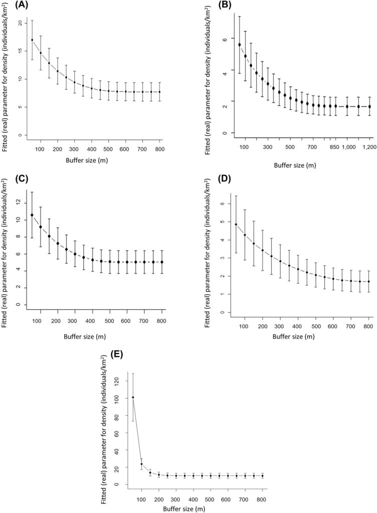
The estimate of density of male roe deer as a function of the buffer width chosen in the spatially explicit capture-recapture analyses using series of null models (M0) integrating the sampling effort. The buffer width chosen for each study area corresponds to the width at which density stabilizes: A) 500 m in Satigny, B) 850 m in Versoix, C) 450 m in Jussy, D) 700 m Chancy, and E) 350 m Jorat, Switzerland, 2018–2020.
APPENDIX C:
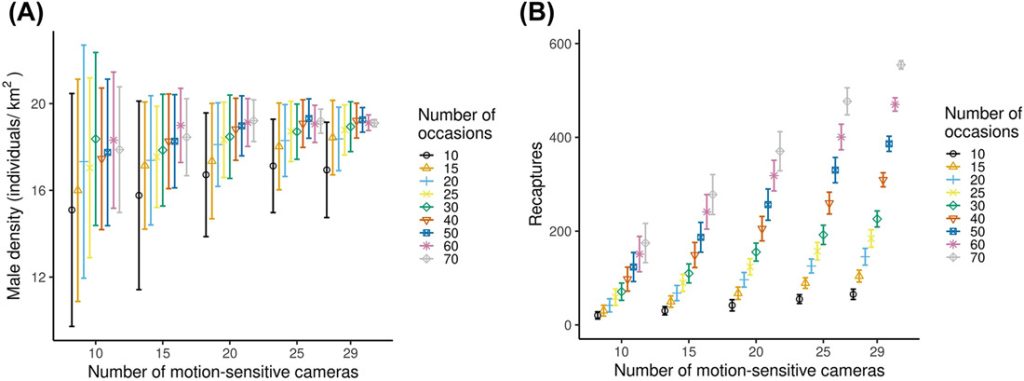
Variation of A) male roe deer density (±SD) and B) recapture of male roe deer (±SD) with increasing sampling effort (from 10 cameras and 10 occasions to 29 cameras and 70 occasions). Models always converged, except for the 10 cameras and 10 occasions combination, where the convergence was 99%. We collected data using motion-sensitive cameras during the pilot survey in Satigny, canton of Geneva, Switzerland, 2018.
APPENDIX C:
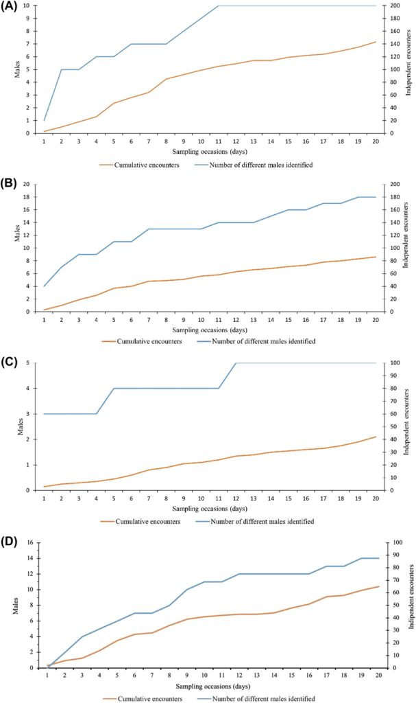
Cumulative number of independent encounters of male roe deer (orange line) and different males identified (blue line) with increasing number of sampling occasions (nights) for A) Versoix, B) Jussy, C) Chancy, and D) Jorat, Switzerland, 2019–2020.
Open Research
DATA AVAILABILITY STATEMENT
The code and data can be made available on request.
REFERENCES
Andersen, J. 1953. Analysis of a Danish roe–deer population (Capreolus capreolus (L.)) based upon the extermination of the total stock. Danish Review of Game Biology 2: 127– 155.Google Scholar
Andersen, R., P. Duncan, and J. D. Linnell. 1998. The European roe deer: the biology of success. Scandinavian European Press, Oslo, Norway.Google Scholar
Baumann, M., H.-A. Meister, J. Muggli, D. Thiel, C. Thiel-Egenter, M. Thürig, P. Volery, P. A. Widmer, and U. Zimmermann. 2012. Chasser en Suisse, sur la voie du permis de chasse. Conférence des services de la faune, de la chasse et de la pêche de Suisse JFK-CSF-CCP. Salm Verlag, Wohlen/Berne, Switzerland.Google Scholar
Beaver, J. T., C. A. Harper, L. I. Muller, P. S. Basinger, M. J. Goode, and F. T. van Manen. 2016. Current and spatially explicit capture-recapture analysis methods for infrared triggered camera density estimation of white-tailed deer. Journal of the Southeastern Association of Fish and Wildlife Agencies 3: 195– 202.Google Scholar
Bessone, M., H. S. Kühl, G. Hohmann, I. Herbinger, K. P. N′Goran, P. Asanzi, P. B. Da Costa, V. Dérozier, E. D. B. Fotsing, B. I. Beka, et al. 2020. Drawn out of the shadows: surveying secretive forest species with camera trap distance sampling. Journal of Applied Ecology 57: 963– 974.Wiley Online LibraryWeb of Science®Google Scholar
Bivand, R., T. Keitt, and B. Rowlingson. 2019. rgdal: bindings for the ‘geospatial’ data abstraction library. https://CRAN.R-project.org/package=rgdalGoogle Scholar
Bobrowski, M., B. Gillich, and C. Stolter. 2020. Nothing else matters? Food as a driving factor of habitat use by red and roe deer in winter? Wildlife Biology 4: wlb.00723.Google Scholar
Borchers, D. L., and M. G. Efford. 2008. Spatially explicit maximum likelihood methods for capture-recapture studies. Biometrics 64: 377– 385.Wiley Online Library | CASPubMedWeb of Science® | Google Scholar
Burbaite, L., and S. Csányi. 2009. Roe deer population and harvest changes in Europe. Estonian Journal of Ecology 58: 169– 180.Crossref | Google Scholar
Burton, A. C., E. Neilson, D. Moreira, A. Ladle, R. Steenweg, J. T. Fisher, E. Bayne, and S. Boutin. 2015. Wildlife camera trapping: a review and recommendations for linking surveys to ecological processes. Journal of Applied Ecology 52: 675– 685.Wiley Online Library | Web of Science® | Google Scholar
Caravaggi, A., M. Zaccaroni, F. Riga, S. C. Schai-Braun, J. T. A. Dick, W. I. Montgomery, and N. Reid. 2016. An invasive-native mammalian species replacement process captured by camera trap survey random encounter models. Remote Sensing in Ecology and Conservation 2: 45– 48.Wiley Online Library | Web of Science® | Google Scholar
Carbone, C., S. Christie, K. Conforti, T. Coulson, N. Franklin, J. Ginsberg, M. Griffiths, J. Holden, K. Kawanishi, M. Kinnaird, et al. 2001. The use of photographic rates to estimate densities of tigers and other cryptic mammals. Animal Conservation 4: 75– 79.Wiley Online Library | Web of Science® | Google Scholar
Cargnelutti, B., D. Reby, L. Desneux, J. M. Angibault, J. Joachim, and A. J. M. Hewison. 2002. Space use by roe deer in a fragmented landscape some preliminary results. Revue d’Écologie 57: 29– 37.Web of Science® | Google Scholar
Chandler, R. B., and A. J. Royle. 2013. Spatially explicit models for inference about density in unmarked or partially marked populations. Annals of Applied Statistics 7: 936– 954.Crossref | Web of Science® | Google Scholar
Chećko, E. 2011. Estimating forest ungulate populations: a review of methods. Forest Research Papers 72: 253– 265.Crossref | Google Scholar
Choo, Y. R., E. P. Kudavidanage, T. R. Amarasinghe, T. Nimalrathna, M. A. H. Chua, and E. L. Webb. 2020. Best practices for reporting individual identification using camera trap photographs. Global Ecology and Conservation 24:e01294.Crossref | Web of Science® | Google Scholar
Dunnington, D. 2017. prettymapr: scale bar, north arrow, and pretty margins in R. https://CRAN.R-project.org/package=prettymapr | Google Scholar
Efford, M. G. 2004. Density estimation in live-trapping studies. Oikos 106: 598– 610.Wiley Online Library | Web of Science® | Google Scholar
Efford, M. G. 2020. secr: spatially explicit capture-recapture models. R package version 4.3.1. https://CRAN.R-project.org/package=secr | Google Scholar
Efford, M. G., and J. Boulanger. 2019. Fast evaluation of study designs for spatially explicit capture–recapture. Methods in Ecology and Evolution 10: 1529– 1535.Wiley Online Library | Web of Science® | Google Scholar
Efford, M. G., and R. M. Fewster. 2013. Estimating population size by spatially explicit capture–recapture. Oikos 122: 918– 928.Wiley Online Library | Web of Science® | Google Scholar
Efford, M. G., and C. M. Hunter. 2018. Spatial capture–mark–resight estimation of animal population density. Biometrics 74: 411– 420.Wiley Online Library | PubMed | Web of Science® | Google Scholar
ENETWILD consortium, S. Grignolio, M. Apollonio, F. Brivio, J. Vicente, P. Acevedo, P. Palencia, K. Petrovic, and O. Keuling. 2020. Guidance on estimation of abundance and density data of wild ruminant population: methods, challenges, possibilities. EFSA Supporting Publication 17: EN- 1876.Google Scholar
Evcin, O., O. Kucuk, and E. Akturk. 2019. Habitat suitability model with maximum entropy approach for European roe deer (Capreolus capreolus) in the Black Sea Region. Environmental Monitoring and Assessment 191: article 669.Crossref | PubMed | Web of Science® | Google Scholar
Federal Office of Meteorology and Climatology. 2022. Measurement values. <https://www.meteoswiss.admin.ch/home/measurement-values.html?param=messwerte-lufttemperatur-10min>. Accessed 12 May 2022.Google Scholar
Findlay, A. M., R. A. Briers, and P. J. C. White. 2020. Component processes of detection probability in camera-trap studies: understanding the occurrence of false-negatives. Mammal Research 65: 167– 180.Crossref | Web of Science® | Google Scholar
Focardi, S., E. Pelliccioni, R. Petrucco, and S. Toso. 2001. Spatial patterns and density dependence in the dynamics of a roe deer (Capreolus capreolus) population in central Italy. Oecologia 130: 411– 419.Crossref | Web of Science® | Google Scholar
Fruziński, B., L. Łabudzki, and M. Wlazełko. 1983. Habitat, density and spatial structure of the forest roe deer population. Acta Theriologica 28: 243– 258.CrossrefGoogle Scholar
Harrell, F. E., Jr. 2022. Hmisc: Harrell miscellaneous. https://CRAN.R-project.org/package=Hmisc | Google Scholar
Henrich, M., F. Hartig, C. F. Dormann, H. S. Kühl, W. Peters, F. Franke, T. Peterka, P. Šustr, and M. Heurich. 2022. Deer behavior affects density estimates with camera traps, but is outweighed by spatial variability. Frontiers in Ecology and Evolution 10:881502.Crossref | Web of Science® | Google Scholar
Heurich, M., K. Zeis, H. Küchenhoff, J. Müller, E. Belotti, L. Bufka, and B. Woelfing. 2016. Selective predation of a stalking predator on ungulate prey. PLoS ONE 11:e0158449.Crossref | PubMed | Web of Science® | Google Scholar
Hewison, A. J. M., and J. M. Gaillard. 1996. Birth-sex ratios and local resource competition in roe deer, Capreolus capreolus. Behavioral Ecology 7: 461– 464.CrossrefWeb of Science® | Google Scholar
Hofmeester, T. R., J. P. G. M. Cromsigt, J. Odden, H. Andrén, J. Kindberg, and J. D. C. Linnell. 2019. Framing pictures: a conceptual framework to identify and correct for biases in detection probability of camera traps enabling multi-species comparison. Ecology and Evolution 9: 2320– 2336.Wiley Online Library | PubMed | Web of Science® | Google Scholar
Howe, E. J., S. T. Buckland, M.-L. Després-Einspenner, and H. S. Kühl. 2017. Distance sampling with camera traps. Methods in Ecology and Evolution 8: 1558– 1565.Wiley Online Library | Web of Science® | Google Scholar
Jennelle, C. S., M. C. Runge, and D. I. MacKenzie. 2002. The use of photographic rates to estimate densities of tigers and other cryptic mammals: a comment on misleading conclusions. Animal Conservation 5: 119– 120.Wiley Online Library | Web of Science® | Google Scholar
Jiménez, J., C. Rodríguez, and Á. Moreno. 2013. Estima de una población de corzo mediante modelos de captura-recaptura clásicos y espacialmente explícitos. Galemys 38: 1– 12.Crossref | Google Scholar
Kaluzinski, J. 1982. Dynamics and structure of a field roe deer population. Acta Theriologica 27: 449– 455.Crossref | Web of Science® | Google Scholar
Karanth, K. U. 1995. Estimating tiger Panthera tigris populations from camera-trap data using capture-recapture models. Biological Conservation 71: 333– 338.Crossref | Web of Science® | Google Scholar
Kjellander, P., A. J. M. Hewison, O. Liberg, J.-M. Angibault, E. Bideau, and B. Cargnelutti. 2004. Experimental evidence for density-dependence of home-range size in roe deer (Capreolus capreolus L.): a comparison of two long-term studies. Oecologia 139: 478– 485.Crossref | CASPubMed | Web of Science® | Google Scholar
Kjøstvedt, J. H., A. Mysterud, and E. Østbye. 1998. Roe deer Capreolus capreolus use of agricultural crops during winter in the Lier valley, Norway. Wildlife Biology 4: 23– 31.Wiley Online Library | Web of Science® | Google Scholar
Kristensen, T. V., and A. I. Kovach. 2018. Spatially explicit abundance estimation of a rare habitat specialist: implications for SECR study design. Ecosphere 9:e02217.Wiley Online Library | Web of Science® | Google Scholar
Lemon, J. 2006. Plotrix: a package in the red light district of R. R-News 6(4): 8– 12.Google Scholar
Macaulay, L. T., R. Sollmann, and R. H. Barret. 2020. Estimating deer populations using camera traps and natural marks. Journal of Wildlife Management 84: 301– 310.Wiley Online Library | Web of Science® | Google Scholar
Mahmoodi, S., A. Alizadeh Shabani, M. Zeinalabedini, O. Khalilipour, and S. Ashrafi. 2020. Identifying habitat patches and suitability for roe deer (Capreolus capreolus) as a protected species in Iran. Caspian Journal of Environmental Sciences 18: 357– 366.Google Scholar
Marcon, A., D. Battocchio, M. Apollonio, and S. Grignolio. 2019. Assessing precision and requirements of three methods to estimate roe deer density. PLoS ONE 14:e0222349.Crossref | CAS | PubMedWeb of Science® | Google Scholar
Martin, J., G. Vourc′h, N. Bonnot, B. Cargnelutti, Y. Chaval, B. Lourtet, M. Goulard, T. Hoch, O. Plantard, A. J. M. Hewison, et al. 2018. Temporal shifts in landscape connectivity for an ecosystem engineer, the roe deer, across a multiple-use landscape. Landscape Ecology 33: 937– 954.Crossref | Web of Science® | Google Scholar
Maublanc M.-L., E. Bideau, R. Willemet, C. Bardonnet, G. Gonzalez, L. Desneux, N. Cèbe, and J.-F. Gerard. 2012. Ranging behaviour of roe deer in an experimental high-density population: are females territorial? Comptes Rendus Biologies 335: 735– 743.Crossref | PubMed | Web of Science® | Google Scholar
McClintock, B. T., and G. C. White. 2009. A less field-intensive robust design for estimating demographic parameters with mark–resight data. Ecology 90: 313– 320.Wiley Online Library | PubMedWeb of Science® | Google Scholar
McClintock, B.T., G. C. White, M. F. Antolin, and D. W. Tripp. 2009. Estimating abundance using mark–resight when sampling is with replacement or the number of marked individuals is unknown. Biometrics 65: 237– 246.Wiley Online Library | PubMedWeb of Science® | Google Scholar
McClintock, B. T., G. C. White, and K. P. Burnham. 2006. A robust design mark-resight abundance estimator allowing heterogeneity in resighting probabilities. Journal of Agricultural, Biological, and Environmental Statistics 11: 231– 248.Crossref | Web of Science® | Google Scholar
Melis, C., B. Jedrzejewska, M. Apollonio, K. A. Barton, W. Jedrzejewski, J. D. C. Linnell, I. Kojola, J. Kusak, M. Adamic, S. Ciuti, I. Delehan, I. Dykyy, K. Krapinec, L. Mattioli, et al. 2009. Predation has a greater impact in less productive environments: variation in roe deer, Capreolus capreolus, population density across Europe. Global Ecology and Biogeography 18: 724– 734.Wiley Online Library | Web of Science® | Google Scholar
Meriggi, A., F. Sotti, P. Lamberti, and N. Gilio. 2008. A review of the methods for monitoring roe deer European populations with particular reference to Italy. Hystrix 19: 103– 120.Web of Science® | Google Scholar
Molinari-Jobin, A., F. Zimmermann, A. Ryser, P. Molinari, H. Haller, C. Breitenmoser Würsten, S. Capt, R. Eyholzer, and U. Breitenmoser. 2007. Variation in diet, prey selectivity and home-range size of Eurasian lynx Lynx lynx in Switzerland. Wildlife Biology 13: 393– 405.Wiley Online Library | Web of Science® | Google Scholar
Morellet, N., F. Klein, E. Solberg, and R. Andersen. 2011. The census and management of populations of ungulates in Europe. Pages 106– 143 in R. Putman, M. Apollonio, and R. Andersen, editors. Ungulate management in Europe: problems and practices. Cambridge University Press, Cambridge, United Kingdom.Crossref | Google Scholar
Mysterud, A. 1999. Seasonal migration pattern and home range of roe deer (Capreolus capreolus) in an altitudinal gradient in southern Norway. Journal of Zoology 247: 479– 486.Wiley Online Library | Web of Science® | Google Scholar
Nichols, J. D., A. F. O′Connell, and K. U. Karanth. 2011. Camera traps in animal ecology and conservation: what’s next? Pages 253– 263 in A. F. O′Connell, J. D. Nichols, and K. U. Karanth, editors, Camera traps in animal ecology: methods and analyses. Springer, New York, New York, USA.Crossref | Web of Science® | Google Scholar
Noon, B. R., L. L. Bailey, T. D. Sisk, and K. S. McKelvey. 2012. Efficient species-level monitoring at the landscape scale. Conservation Biology 26: 432– 441.Wiley Online Library | PubMed | Web of Science® | Google Scholar
Norouzzadeh, M. S, D. Morris, S. Beery, N. Joshi, N. Jojic, and J. Clune. 2021. A deep active learning system for species identification and counting in camera trap images. Methods in Ecology and Evolution 12: 150– 161.Wiley Online Library | Web of Science® | Google Scholar
O′Brien, T. G., M. F. Kinnaird, and H. T. Wibisono. 2003. Crouching tigers, hidden prey: Sumatran tiger and prey populations in a tropical forest landscape. Animal Conservation 6: 131– 139.Wiley Online Library | PubMed | Web of Science® | Google Scholar
O′Connell, A. F., J. D. Nichols, and K. U. Karanth. 2011. Camera traps in animal ecology: methods and analyses. Springer, New York, New York, USA.Crossref | Web of Science® | Google Scholar
Otis, D. L., K. P. Burnham, G. C. White, and D. R. Anderson. 1978. Statistical inference from capture data on closed animal populations. Wildlife Monographs 62: 3– 135.Google Scholar
Parsons, A. W., T. Forrester, W. J. McShea, M. C. Baker-Whatton, J. J. Millspaugh, and R. Kays. 2017. Do occupancy or detection rates from camera traps reflect deer density? Journal of Mammalogy 98: 1547– 1557.Crossref | Web of Science® | Google Scholar
Pebesma, E. J., and R. S. Bivand. 2005. Classes and methods for spatial data in R. R News 5(2): 9– 13.Google Scholar
Pfeffer, S. E., R. Spitzer, A. M. Allen, T. R. Hofmeester, G. Ericsson, F. Widemo, N. J. Singh, and J. P. Cromsigt. 2017. Pictures or pellets? Comparing camera trapping and dung counts as methods for estimating population densities of ungulates. Remote Sensing in Ecology and Conservation 4: 173– 183.Wiley Online Library | Web of Science® | Google Scholar
Pielowski, Z. 1984. Some aspects of population structure and longevity of field roe deer. Acta Theriologica 29: 17– 33.Crossref | Web of Science® | Google Scholar
Putman, R., J. Langbein, P. Green, and P. Watson. 2011. Identifying threshold densities for wild deer in the UK above which negative impacts may occur. Mammal Review 41: 175– 196.Wiley Online Library | Web of Science® | Google Scholar
R Core Team. 2019. R: a language and environment for statistical computing. R Foundation for Statistical Computing, Vienna, Austria.Google Scholar
Ratcliffe, P. R. 1987. Red deer population changes and the independent assessment of population sizes. Symposia of the Zoological Society of London 17: 153– 165.Google Scholar
Repucci, J., B. Gardner, and M. Lucherini. 2011. Estimating detection and density of the Andean cat in the high Andes. Journal of Mammalogy 92: 140– 147.Crossref | Web of Science® | Google Scholar
Richard, E., J. M. Gaillard, S. Saïd, J.-L. Hamann, and F. Klein. 2010. High red deer density depresses body mass of roe deer fawns. Oecologia 163: 91– 97.Crossref | PubMed | Web of Science® | Google Scholar
Rodríguez-Morales, B., E. R. Díaz-Varela, and M. F. Marey-Pérez. 2013. Spatiotemporal analysis of vehicle collisions involving wild boar and roe deer in NW Spain. Accident Analysis and Prevention 60: 121– 133.Crossref | PubMed | Web of Science® | Google Scholar
Rovero, F., and A. Marshall. 2009. Camera trapping photographic rate as an index of density in forest ungulates. Journal of Applied Ecology 46: 1011– 1017.Wiley Online Library | Web of Science® | Google Scholar
Rovero, F., and F. Zimmermann. 2016. Camera features related to specific ecological applications. Pages 8– 21 in F. Rovero and F. Zimmermann, editors. Camera trapping for wildlife research. Pelagic Publishing, London, United Kingdom.Google Scholar
Rovero, F., F. Zimmermann, D. Berzi, and P. Meek. 2013. Which camera trap type and how many do I need? A review of camera features and study designs for a range of wildlife research applications. Hystrix 24: 148– 156.Web of Science® | Google Scholar
Rowcliffe, J. M., C. Carbone, P. A. Jansen, R. Kays, and B. Kranstauber. 2011. Quantifying the sensitivity of camera traps: an adapted distance sampling approach. Methods in Ecology and Evolution 2: 464– 476.Wiley Online Library | Web of Science® | Google Scholar
Rowcliffe, J. M., J. Field, S. T. Turvey, and C. Carbone. 2008. Estimating animal density using camera traps without the need for individual recognition. Journal of Applied Ecology 45: 1228– 1236.Wiley Online Library | Web of Science® | Google Scholar
Rowcliffe, J. M., P. A. Jansen, R. Kays, B. Kranstauber, and C. Carbone. 2016. Wildlife speed cameras: measuring animal travel speed and day range using camera traps. Remote Sensing in Ecology and Conservation 2: 84– 94.Wiley Online Library | Web of Science® | Google Scholar
Royle, J. A., A. K. Fuller, and C. Sutherland. 2016. Spatial capture–recapture models allowing Markovian transience or dispersal. Population Ecology 58: 53– 62.Wiley Online Library | Web of Science® | Google Scholar
Royle, J. A., K. U. Karanth, A. M. Gopalaswamy, and N. S. Kumar. 2009a. Bayesian inference in camera-trapping studies for a class of spatial capture–recapture models. Ecology 90: 3233– 3244.Wiley Online Library | PubMed | Web of Science® | Google Scholar
Royle, J. A., J. D. Nichols, K. U. Karanth, and A. M. Gopalaswamy. 2009b. A hierarchical model for estimating density in camera-trap studies. Journal of Applied Ecology 46: 118– 127.Wiley Online Library | Web of Science® | Google Scholar
Royle, J. A., and K. V. Young. 2008. A hierarchical model for spatial capture–recapture data. Ecology 89: 2281– 2289.Wiley Online Library | PubMed | Web of Science® | Google Scholar
Sarkar, D. 2008. Lattice: multivariate data visualization with R. Springer, New York, New York, USA.Crossref | Web of Science® | Google Scholar
Sollmann, R., A. Mohamed, H. Samejima, and A. Wilting. 2013. Risky business or simple solution—relative abundance indices from camera-trapping. Biological Conservation 159: 405– 412.Crossref | Web of Science® | Google Scholar
Spitzer, R., E. Coissac, A. Felton, C. Fohringer, L. Juvany, M. Landman, N. J. Singh, P. Taberlet, F. Widemo, and J. P. G. M. Cromsigt. 2021. Small shrubs with large importance? Smaller deer may increase the moose-forestry conflict through feeding competition over Vaccinium shrubs in the field layer. Forest Ecology and Management 480:118768.Crossref | Web of Science® | Google Scholar
Taylor, J. C., S. B. Bates, J. C. Whiting, B. R. McMillan, and R. T. Larsen. 2020. Optimising deployment time of remote cameras to estimate abundance of female bighorn sheep. Wildlife Research 48: 127− 133.Crossref | Web of Science® | Google Scholar
Taylor, J. C., S. B. Bates, J. C. Whiting, B. R. McMillan, and R. T. Larsen. 2021. Using camera traps to estimate ungulate abundance: a comparison of mark-resight methods. Remote Sensing in Ecology and Conservation 8: 32− 44.Wiley Online Library | Web of Science® | Google Scholar
Therneau, T. 2022. A package for survival analysis in R. R package version 3.3-1. https://CRAN.R-project.org/package=survivalGoogle Scholar
Trolliet, F., M. C. Huynen, V. Cédric, and H. Alain. 2014. Use of camera traps for wildlife studies. A review. Biotechnology, Agronomy, Society and Environment 18: 446– 454.Web of Science®Google Scholar
Vidal, M., N. Wolf, B. Rosenberg, B. P. Harris, and A. Mathis. 2021. Perspectives on individual animal identification from biology and computer vision. Integrative and Comparative Biology 61: 900– 916.Crossref | PubMed | Web of Science® | Google Scholar
Wahlström, L. K. 1994. The significance of male-male aggression for yearling dispersal in roe deer (Capreolus capreolus). Behavioral Ecology and Sociobiology 35: 409– 412.Crossref | Web of Science® | Google Scholar
Wahlström, L. K., and O. Liberg. 1995. Patterns of dispersal and seasonal migration in roe deer (Capreolus capreolus). Journal of Zoology 235: 455– 467.Wiley Online Library | Web of Science® | Google Scholar
White, G. C. 1996. NOREMARK: population estimation from mark-resighting surveys. Wildlife Society Bulletin 24: 50– 52.Web of Science® | Google Scholar
Whittington, J., M. Hebblewhite, and R. B. Chandler. 2017. Generalized spatial mark-resight models with an application to grizzly bears. Journal of Applied Ecology 55: 157– 168.Wiley Online Library | Web of Science® | Google Scholar
Wickham, H. 2016. ggplot2: elegant graphics for data analysis. Springer-Verlag, New York, New York, USA.Google Scholar
Zeileis, A., and Y. Croissant. 2010. Extended model formulas in R: multiple parts and multiple responses. Journal of Statistical Software 34(1): 1– 13.Crossref | Web of Science® | Google Scholar
Zimmermann, F., and D. Foresti. 2016. Capture-recapture methods for density estimation. Pages 95– 141 in F. Rovero and F. Zimmermann, editors. Camera trapping for wildlife research. Pelagic Publishing, London, United Kingdom.Google Scholar